Bayesian Inference
Background: Bayes Rule and Bayesian Inference
Here’s a quick refresher from Wikipedia: “In probability theory and applications, Bayes’s rule relates the odds of events … after (posterior to) conditioning on another event.”
This reads: “the probability of given that is observed is proportional to the probability of times the probability of given that is observed”.
(Note: "...probability of A..." is unconditional on B, i.e. "...the probability of A for all possible values of B...". Also, A is a member of a set possible events or states, and, likewise, B is a member of a different set.)
In even simpler terms, Bayes rule can be used to update our estimate of the probability distribution a random variable (“the prior”) using information from observed events (“conditioning”), to arrive at a better estimate of the distribution (“the posterior”). Wikipedia: “The posterior probability is proportional to prior probability times likelihood.”
Bayesian Networks with Point Probabilities
Often there are conditional relationships among several random variables, and Bayesian Networks are used to represent these relationships. Here is an example:

In this case, we have four random variables: cloudy, sprinklers, rain, and wet grass. The probability of cloudy is 0.5. Given that cloudy = TRUE on a given day, the probability of rain is 0.8, and so on.
Bayesian Inference is the process of using Bayes Rule over and over to modify the prior probabilities, given the actual (observed) values for some other random variables. The model can answer questions like “What is the probability that it is raining, given the grass is wet?” and “What is the probability that it is cloudy, given that the grass is not wet?”.
// Implements the Bayesian Network, above
var grassGetsWet = Infer({ method: 'enumerate' }, function(){
  var cloudy = flip(0.5);
  var rain = cloudy ? flip(0.8) : flip(0.2);
  var sprinkler = cloudy ? flip(0.1) : flip(0.5);
  var wetGrass = rain && sprinkler
                   ? flip(.99)
                   : (rain && !sprinkler) || (!rain && sprinkler)
                        ? flip(0.9)
                        : flip(0.0);
  condition(cloudy === true);
  return wetGrass;
});


print('Probability of wet grass, given cloudy = '
               + Math.exp(grassGetsWet.score(true)) );
// same model conditioned differently, with different return variables
///fold:
// Version 1
var grassGetsWet1 = Infer({ method: 'enumerate' }, function(){
  var cloudy = flip(0.5);
  var rain = cloudy ? flip(0.8) : flip(0.2);
  var sprinkler = cloudy ? flip(0.1) : flip(0.5);
  var wetGrass = rain && sprinkler
                   ? flip(.99)
                   : (rain && !sprinkler) || (!rain && sprinkler)
                        ? flip(0.9)
                        : flip(0.0);
  // no conditions
  return wetGrass;
});

// Version 2
var grassGetsWet2 = Infer({ method: 'enumerate' }, function(){
var cloudy = flip(0.5);
var rain = cloudy ? flip(0.8) : flip(0.2);
var sprinkler = cloudy ? flip(0.1) : flip(0.5);
var wetGrass = rain && sprinkler
                   ? flip(.99)
                   : (rain && !sprinkler) || (!rain && sprinkler)
                        ? flip(0.9)
                        : flip(0.0);
// no conditions
return rain;
});

// Version 3
var grassGetsWet3 = Infer({ method: 'enumerate' }, function(){
  var cloudy = flip(0.5);
  var rain = cloudy ? flip(0.8) : flip(0.2);
  var sprinkler = cloudy ? flip(0.1) : flip(0.5);
  var wetGrass = rain && sprinkler
                   ? flip(.99)
                   : (rain && !sprinkler) || (!rain && sprinkler)
                        ? flip(0.9)
                        : flip(0.0);
  condition(wetGrass === true);
  return rain;
});

// Version 4
var grassGetsWet4 = Infer({ method: 'enumerate' }, function(){
  var cloudy = flip(0.5);
  var rain = cloudy ? flip(0.8) : flip(0.2);
  var sprinkler = cloudy ? flip(0.1) : flip(0.5);
  var wetGrass = rain && sprinkler
                   ? flip(.99)
                   : (rain && !sprinkler) || (!rain && sprinkler)
                        ? flip(0.9)
                        : flip(0.0);
  condition(sprinkler === true);
  return rain;
});


///
print('Probability of wet grass (aka prior) = '
               + Math.exp(grassGetsWet1.score(true)));
print('Probability of rain (aka prior) = '
               + Math.exp(grassGetsWet2.score(true)));
print('Probability of rain, given the grass is wet = '
                + Math.exp(grassGetsWet3.score(true)));
print('Probability of rain, given the sprinkler was on = '
                + Math.exp(grassGetsWet4.score(true)));
Let’s look at this program in detail, built up in steps starting in the middle. This will show you all the basic ingredients for any WebPPL probabilistic program.
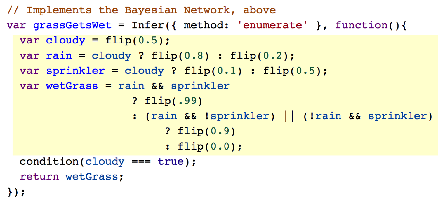
Starting in the middle, the code highlighted in yellow is the generative model that specifies the random variables and their probability distributions. Notice that the logic in this section is simply a transcription of the Bayesian Network, above. Short and simple!
flip(0.5) is a function that draws a sample from a Bernoulli distribution (“true” or “false”), with .
The function “predicate ? if_true : if_false” is “syntatic sugar” for an ifelse( ) function that you might recognize in other languages. It returns if_true statement if predicate is true, and if_false otherwise. This function is very useful and often necessary functional programming to conditionally assign a value of a variable.
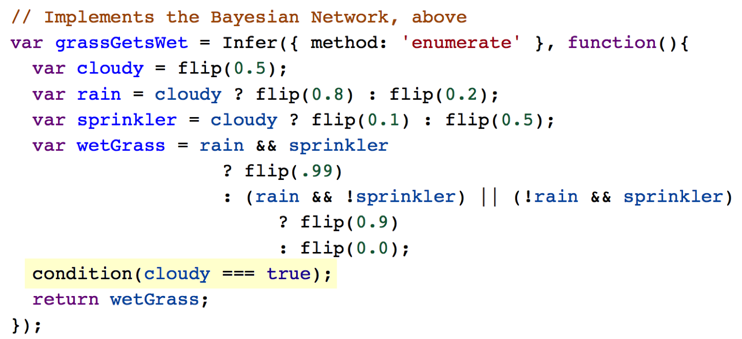
After the generative model is a condition(...); statement. This is how WebPPL introduces observations (a.k.a. empirical data, constraints, etc.). Condition statements are optional.
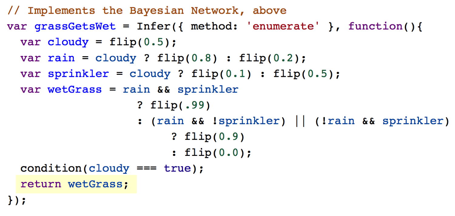
The last statement is a return statement, which is the posterior distribution you are trying to make inferences on.
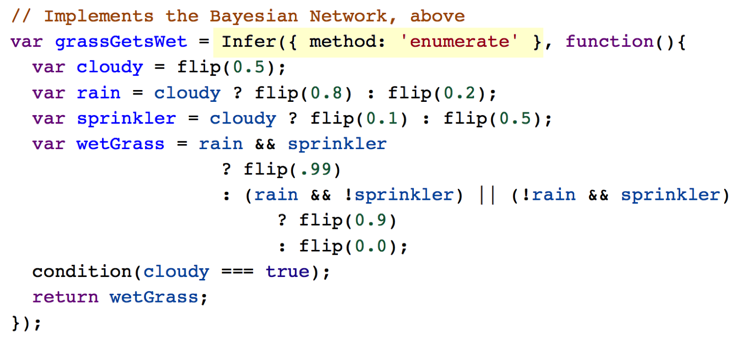
The final ingredient to a WebPPL program is the Infer(...); statement. This function does the “magic” of conditioning the random variables on the observations. It takes two parameters: 1) an inference method (e.g. “Enumerate”); and 2) the generative function that encompasses your model plus observed data (via condition statements.)
A Better Version
The following model is the same as above, but instead of four separate functions with different conditions for evidence, we combine them into one function that takes any combination of evidence and outputs the all marginal probabilities.
You can enter your own evidence combination where it says “ENTER EVIDENCE HERE”.
// Wet Grass causal model

///fold:
// Helper function
var mapToString = function(map){
  var keys = Object.keys(map);
  var mapString = reduce(function(x,acc){
    var sep = acc.length == 0 ? "" : ", "
    return acc.concat(sep + x + " : " + map[x] )
  },"",keys );
  return "{" + mapString + "}";
}

// Generative model
var grassGetsWet = function(){
  var cloudy = flip(0.5);
  var rain = cloudy ? flip(0.8) : flip(0.2);
  var sprinkler = cloudy ? flip(0.1) : flip(0.5);
  var wetGrass = rain && sprinkler
                   ? flip(.99)
                   : (rain && !sprinkler) || (!rain && sprinkler)
                        ? flip(0.9)
                        : flip(0.0001); // what is the prob. of some
                                        //   other cause, not in model?
                              // was flip(0.0); // impossibility
  return {wetGrass: wetGrass,
          rain: rain,
          sprinkler: sprinkler,
          cloudy: cloudy};
}

// Generalized inference function given any combination of evidence
var inference = function(evidence){
  var applyEvidence = Infer({ method: 'enumerate' }, function(){
  var trial = grassGetsWet();
   if ("sprinkler" in evidence){
      condition(trial.sprinkler === evidence.sprinkler);
   }
   if ("rain" in evidence){
      condition(trial.rain === evidence.rain);
   }
   if ("cloudy" in evidence){
      condition(trial.cloudy === evidence.cloudy);
   }
   if ("wetGrass" in evidence){
      condition(trial.wetGrass === evidence.wetGrass);
   }
   return {rain: trial.rain,
           cloudy: trial.cloudy,
           sprinkler: trial.sprinkler,
           wetGrass: trial.wetGrass,
          };
});

  return applyEvidence;
}
///

// ENTER EVIDENCE HERE in this form:
//      { cloudy : true,
//          rain : false }
// Leave out any entry where there is no evidence

var evidence = {cloudy : false,
               wetGrass: true};

var evidenceString = mapToString(evidence);

// Output
print("Given evidence = " + mapToString(evidence) + " =>");
var allCombinations = inference(evidence);

// Extract marginal probabilities:
///fold:
var results = {
  rain: Math.exp(
                 Infer({method: 'enumerate'},
                   function(){
                      var trial = sample(allCombinations);
                      return trial.rain;
                   }
                 ).score(true)
               ),
  cloudy: Math.exp(
                 Infer({method: 'enumerate'},
                   function(){
                      var trial = sample(allCombinations);
                      return trial.cloudy;
                   }
                 ).score(true)
               ),
  wetGrass: Math.exp(
                 Infer({method: 'enumerate'},
                   function(){
                      var trial = sample(allCombinations);
                      return trial.wetGrass;
                   }
                 ).score(true)
               ),
  sprinkler: Math.exp(
                 Infer({method: 'enumerate'},
                   function(){
                      var trial = sample(allCombinations);
                      return trial.sprinkler;
                   }
                 ).score(true)
               )
}
///

print(" => Pr(rain) = " + results.rain);
print("    Pr(cloudy) = " + results.cloudy);
print("    Pr(wetGrass) = " + results.wetGrass);
print("    Pr(sprinkler) = " + results.sprinkler);

print("\nAll state combinations");

viz.table(allCombinations);
It’s worth looking at the code below “Extract marginal probabilities”. Since our inference(evidence) function is we are returning all four state variables rather than one, and because Infer returns a distribution object, what we get is a distribution over all state combinations. Therefore, to eextract the marginal distributions (i.e. unconditioned), e.g. regardless of other states, we need to apply Infer to allCombinations, each time returning a different state variable, converting that to a score (log value), then transforming it into probability via exponential function.
Bayesian Inference With Continuous Distributions
Most examples and lessons on Bayesian Inference use point probabilities. The same rules and principles apply for continuous probiability distributions, but the math gets much, much harder if the underlying distributions are anything but simple (i.e Uniform, Gaussian, and related).
First, let us look at a textbook example: a single random variable with prior uniform distribution that is conditioned by set of observations drawn from a (truncated) Gaussian. You can find this example in textbooks because it admits to a “closed form solution”.
// x is a random variable with a uniform prior distribution
var genX = function(){
   return uniform(0,10);
}

var generatePrior = Infer({method: 'SMC', particles: 1000, rejuvSteps: 5},
    function() { return genX();}
);

// This function generates the observational data from a simple distribution
var obs = function(){
var x = gaussian({mu: 6, sigma: 1});
condition(x >= 0);
condition(x <= 10.0);
return x;
}

var generateObservations = Infer({method: 'SMC', particles: 1000, rejuvSteps: 5},
function(){
return obs();
});

// Infer the posterior distribution, give the observations
var generateXconditioned = function(logWeightOfEvidence){
var w = - logWeightOfEvidence;
return Infer({method: 'SMC', particles: 1000, rejuvSteps: 5},
function(){
var x = genX();
var ob = obs();
factor(ob - 0.1 < x && ob + 0.1 > x ? 0 : w );
return x;
});}

print("Prior distribution");
viz.auto(generatePrior);
print("Observations distribution");
viz.auto(generateObservations);
print("Weak weight of observations");
viz.auto(generateXconditioned(1));
print("Strong weight of observations");
viz.auto(generateXconditioned(4));
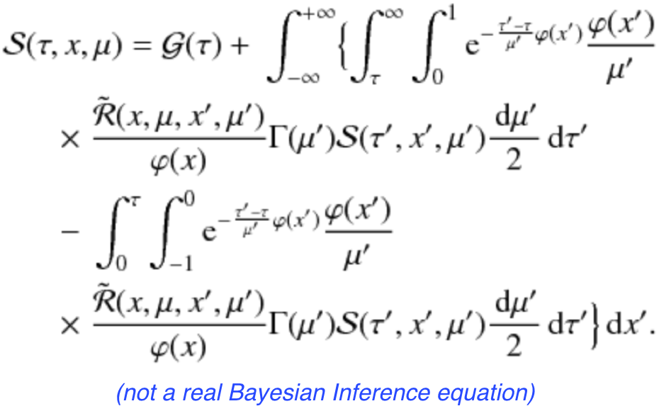
But when the distributions aren’t simple or “nice”, the math gets messy real fast, looking something like this:
In the next code window is essentially the same program, but with more complex distributions. Notice that the program is not really much more complex, and the execution times (complile and run) are about the same.
// x is a random variable with a complex prior distribution
var genX = function(){
var y = gaussian({mu: -1, sigma: 1});
var z = gaussian({mu: 1, sigma: 3});
var x = y >= z ? uniform(0,4) : uniform(5,10);
return x;
}

var generatePrior = Infer({method: 'SMC', particles: 1000, rejuvSteps: 5},
function() { return genX();}
);

// This function generates the observational data from a complex distribution
var obs = function(){
var y = gaussian({mu: 0, sigma: 3});
var z = gaussian({mu: 1, sigma: 3});
var x = y >= z ? cauchy(4, .5) : gamma(1, 2);
condition(x >= 0);
condition(x <= 10.0);
return x;
}

var generateObservations = Infer({method: 'SMC', particles: 1000, rejuvSteps: 5},
function(){
return obs();
});

// Infer the posterior distribution, give the observations
var generateXconditioned = function(logWeightOfEvidence){
var w = - logWeightOfEvidence;
return Infer({method: 'SMC', particles: 1000, rejuvSteps: 5},
function(){
var x = genX();
var ob = obs();
factor(ob - 0.1 < x && ob + 0.1 > x ? 0 : w );
return x;
});}

print("Prior distribution");
viz.auto(generatePrior);
print("Observations distribution");
viz.auto(generateObservations);
print("Weak weight of observations");
viz.auto(generateXconditioned(1));
print("Strong weight of observations");
viz.auto(generateXconditioned(4));
To Do
- Add a section on Bayesian model fitting, using the synthetic time series.
- Maybe add one or two models from the “Puppy Book”.
- Add a Conclusion section.