Empirical Bayesian Analysis
Empirical Bayesian data analysis are a set of methods that are an attractive alternative to frequentist methods, e.g. Null Hypothesis Significance Testing, linear regression, logistic regression, Analysis of Variance (ANOVA). Though there are specialized tools (e.g. STAN) for Bayesian data analysis, this use case shows the versitility and general applicablity of probabilistic programming.
Testing the Fairness of a Coin With Limited Information
How many coin tosses do you need to see before you can decide whether a coin is fair or unfair?
Imagine that someone tosses a coin once…twice…three times and you see three “heads” in a row. Is that strong evidence that the coin is unfair (not 50/50)? How many more consecutive “heads” would you need to see to decide whether this was a fair or unfair coin?
Checking whether a coin is fair is a “a simple problem on which to illustrate basic ideas of statistical inference also provides a simple problem that can be used to compare various competing methods of statistical inference”* given limited information.
*Wikipedia has a nice article here, including comparison of the Bayesian approach (fixed number of tosses plus prior knowledge) vs the Frequentist approach (any number of tosses and no prior knowledge)
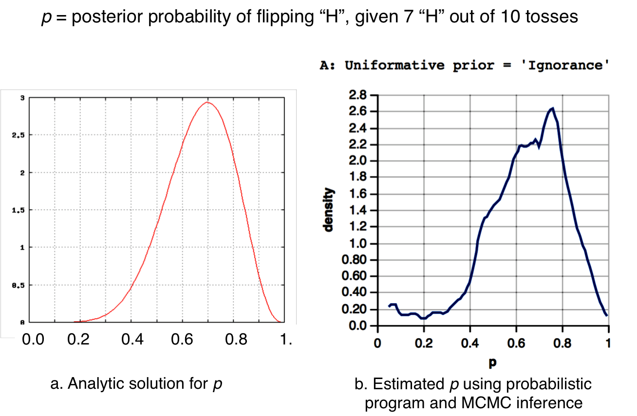
Though this problem is simple enough to calculate probabilities analytically, it makes a nice problem to start demonstrating how probabilistic programming can be used for empirical data analysis and empirical inference, in part because we can compare our results with the exact results from analysis. For example, here are two plots with the same conditions: prior = uniform distribution, with evidence of 7 heads out of 10 tosses. On the left is the analytical solution, and on the right is output from the program below.
What is “Fair”? (A bit of subjectivity)
While we commonly think of a fair coin as having exactly 0.5 probability of heads, this is an idealization that assumes that we can (or must) toss the coin very many times (arbitrarily many). If we know ahead of time that we will only toss the coin a few or many times, we may accept a coin as “fair” of the probability of heads is close to 0.5. How close? This depends on the decision maker and what you will do with the information. Are you placing bets? Are you comparing coins, to chose the most fair (or unfair)?
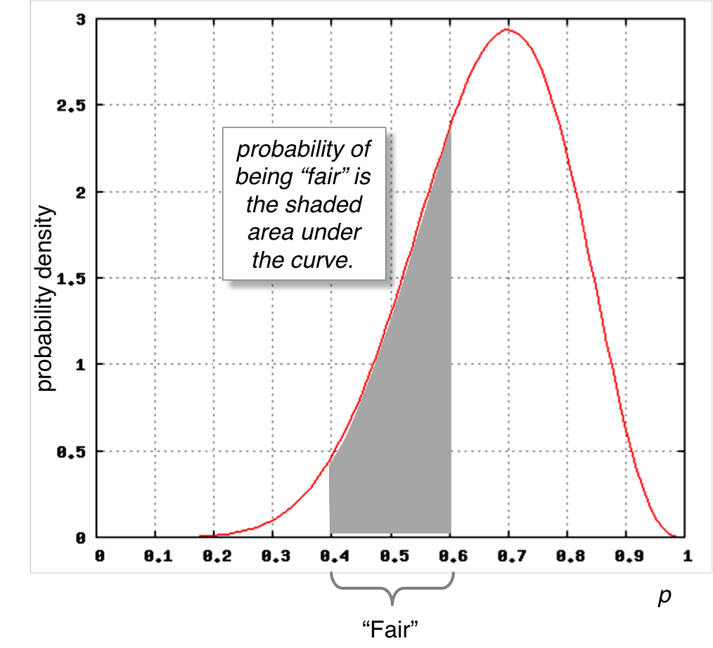
In our case, we’ll define “fair” as . The probability that a coin is fair given the probability distribution of heads, , is defined as the area under the curve between the limits 0.4 and 0.6, as shown in the figure below.
"...area under the curve...": This is why probability and statistics requries calculus once you start dealing with continuous probability distributions. Notice that if we only accepted p = 0.5 as "fair", then the shaded area would be zero!
What if this were a uniform (flat) distribution? Then the probability of a fair coin would be quite low, because much more probability mass lies outside that range than inside. Think about this for a few seconds. Analysts and modelers are often inclined to use uniform distributions as prior distributions if the random variable is bounded (in this case ), because it feels safer to not assume anything about the likely value of . But the implication, in this case, is that you are also making a fairly strong assumption that most coins are biased. If you only have a little evidence (i.e. a few tosses), that could lead to some weird inferences and decisions.
The reverse would be true if your prior or posterior distribution were narrow and concentrated within the “fair” range. You’ll see these effects in the experiment that follows.
Bayesian Analysis of Coin Tossing Experiment
Here’s the experimental setup. There are K total coin tosses, with numH = number of heads (“H”) out of K, but only the first N will be observed. Thus K defines the “longest possible run” or “all possible data” and the ratio numH / K is the “ground truth” of the probability of tossing “heads” (a.k.a. ). If is close to 0.5, then the coin is fair.
To execute the program and generate results, click button below the codebox that follows.
Initially K = 10; N = 10; numH = 7, therefore . When , that means you are seeing all of the available data. If , you are only seeing some of it. You can set these to any positive integer as long as ; and ; . Try setting N = 1 (a single toss), or N = 3, or set K to a large number, with proportionate numH.
Three Models With Different Prior Distributions
Notice what happens in each of these settings with the three cases of prior knowledge: 1) uninformed (uniform distribution); 2) somewhat informed (beta distribution); and 3) very informed (narrow Gaussian distribution).
Code and comments that are less important in understanding the experiment is hidden by the `///fold:` macro. To view this code, simply click on the button in the codebox.
//************************
// UTILITY FUNCTIONS
//************************
//   count(item,arr); takeN(n, arr); shuffle(arr), truncatedGaussian()
///fold:
// count: count the number of "item" in "arr"
var count = function(item,arr){
    if (arr.length === 0 || item.length === 0){
       return 0;
    } else {
      return filter(function(x){return x == item;},arr).length;
    }
}

// takeN: return the first "n" elements of "arr"
var takeN = function(n, arr){
    return n <= 0 || arr.length === 0
        ? 0
        : remove(null, mapIndexed(function(i,x){return i < n ? x : null},arr));
}

var removeIndexed = function(i, arr){
    return remove(null,mapIndexed(function(j,x){return j === i ? null : x;}, arr));
}

// add random elements from array to an accumulator
//  This is a recursive function, with safety counter
var addRandomElement = function(arr,acc,count){
    if (count >= 0 && arr.length > 0){
        var x = sample(RandomInteger({n:arr.length}));
        var newAcc = acc.concat(arr[x]);
        var newArr = removeIndexed(x,arr);
        var newCount = count - 1;
        addRandomElement(newArr,newAcc,newCount);
    } else {
        return acc;
    }
}

// shuffle: return an array in random order
var shuffle = function(arr){
    return addRandomElement(arr,[],arr.length);
}
// truncatedGaussian: returns a distribution with mean mu and s.d. sigma,
//   truncated at 0.0 and 1.0, inclusive
var truncatedGaussian = function(mu, sigma){
    var x = gaussian({mu:mu,sigma:sigma});
    condition(x >= 0 && x <= 1.0);
    return x;
}
///

//************************
// EXPERIMENT PARAMETERS
//************************

var K = 10; // total number of observations in trial
var numH = 7; // number of Heads in all observations in the trial
var N = 10; // number of (randomly selected) observations in observedData

//************************
// OBSERVED DATA ("EVIDENCE")
//************************
var trial = mapN(function(x){return x < numH ? "H": "T";},K);
var observations = shuffle(trial);
var observedData = takeN(N,observations);
var obsH = count("H", observedData);

//************************
// PRIOR KNOWLEDGE
//************************

// Uniformative prior:
///fold:
//    We have no expectation of likelihood of fair coins vs unfair coins
//  Therefore, a uniform(0,1) fits this lack of prior knowledge
///
var uninformativePrior = function(){return uniform(0,1);}

// Somewhat informative prior:
///fold:
//    We expect fair coins to be most common: mean = 0.5;
//    Equal probability of unfairness in both H and T;
//    With declining probability as p -> 1 and -> 0;
//    Zero probability of deterministic coin (always H or T)
//  Therefore, a Beta(2,2) fits this prior knowledge.
///
var informativePrior = function(){return beta(2,2);}

// Very informative prior:
///fold:
//    We expect fair coins to be most common: mean = 0.5;
//    Equal probability of unfairness in both H and T;
//    Unfair coins are very rare, especially at extremes.
//    Zero probability of deterministic coin (always H or T)
//  Therefore, a Gaussian(0.5,0.1) fits this prior knowledge.
///
var highlyInformativePrior = function(){return truncatedGaussian(0.5,0.1);}

//************************
// MODEL and INFERENCE
//************************

// toss: function that returns "H" with probability r, otherwise "T"
var toss = function(r) {return flip(r) ? "H" : "T";}

// We'll use MCMC inference, since our variable of interest is continuous with
//  finite support (0,1), and without multiple modes or other complications.
var mcmcParms = {method: 'MCMC', kernal : "MH", samples:25000, burn: 1000};
var posterior = function(prior) {
    return Infer(mcmcParms,
        function () {
            //  p is defined as the probability of "H" on a single toss,
            //  in the range (0,1). p is our variable of interest
            var p = prior();
            // data: N random draws from toss(p), given random draw of p
            var data = repeat(N,function(){return toss(p);});
            // Count the number of heads, since we don't care about the order
            var dataH = count("H",data);
            // Upweight likelihood when # of "H" in data = # of "H" in observed
            observe(Gaussian({mu: dataH, sigma: 0.2}), obsH);
            // ^^^^^ try commenting this out, and uncomment "factor(...)" below

            // "factor()" is a second method for weighting likelihood.
            //   This is a "softer" method because it downweights non-matching
            //   execution traces by an amount proportional to the number of tosses,
            //   as opposed to downweight by -Infinity, as in condition() and observe().
            //   The justification is that with few tosses, you have less justification
            //   for modifying your prior beliefs
            // factor (dataH == obsH ? 0 : -( N / 2.5));
            //  ^^^^^ try uncommenting this,
            //          while also commenting out "observe(...)" above
            return {p: p};
        });
}

//************************
// FAIR COIN INFERENCE: Is it fair, given prior knowledge and evidence?
//************************

var upperLimit = 0.6;
var lowerLimit = 0.4;
var options = {method: 'forward', samples: 5000}

var fairTest = function(dist,lower,upper){
    return Infer(options,function() {
        var A = sample(dist);
        var D = (A.p >= lower && A.p <= upper);
        return {"fair?" : D};
    });
}

//************************
// RUN MODELS AND VISUALIZE RESULTS
//************************
///fold:

var trialString = "(Observe " + obsH +" heads in "+ N +" tosses)";
var trialA = posterior(uninformativePrior);
var fairA = fairTest(trialA,lowerLimit,upperLimit);

print("A: Uniformative prior = 'Ignorance' "  + trialString);
viz.auto(trialA);
viz.auto(fairA);


var trialB = posterior(informativePrior);
var fairB = fairTest(trialB,lowerLimit,upperLimit);
print("B: Somewhat Informative prior = 'Most coins are fair' "+ trialString);
viz.auto(trialB);
viz.auto(fairB);

var trialC = posterior(highlyInformativePrior);
var fairC = fairTest(trialC,lowerLimit,upperLimit);
print("C: Highly Informative prior = 'Nearly all coins are fair' "+ trialString);
viz.auto(trialC);
viz.auto(fairC);
///
Analysis of results – With the default parameters (7 of 10 tosses are “H”), you’ll notice first that all three inference queries returned a mean estimate for that is above 0.5, suggesting that the coin is biased toward heads. But the statistical test for fairness returns different results in all three. Model A (Uninformative prior) puts most of the probability on (about 0.75). Model B (Somewhat informative prior) is about the same. But Model C (Very informative prior) returns the opposite result, where has probability of about 0.69.
Why?
Because, of the three models, Model C is the most resistant to change with new information. In a sense, it takes a lot of evidence to pull it off the prior knowledge (assumption) that nearly all coins are fair. In contrast, Model A is most easily swayed by even a fragment of evidence. To see this, change N = 1; (a single coin toss)and click button again.
You’ll see the probability density function (PDF) output for in Model A is dramatically affected, while Model B output is somewhat affected, and Model C output is hardly affected. As Bayesian analysts and modelers, we should always be thinking:
How Much Influence Should Evidence Have?
(more subjectivity)
What ever model, conditioning, and inference methods you use, you should always be conscious of how much influence observations (evidence, constraints, etc.) will have on prior distributions. As mentioned in previous chapters, the Infer() function is used by WebPPL to tally likelihood weights for all (or nearly all common) traces of your model (i.e. the rest of the program). Functions like observe(), condition(), and factor() perform the likelihood weighting operations. In the default configuration, we use an observe(...) function:
observe(Gaussian({mu: dataH, sigma: 0.2}), obsH);
…which does this: “set the likelihood for the current trace high if the observed number of heads obsH is approximately the same as the data (number of heads) generated by this trace dataH, with a small Gaussian noise term; Otherwise set likelhood to a low value.”
This approach has some benefits but also negatives. For example, it does not take into account the amount of evidence, i.e. number of tosses . Most people have the intuition that a single toss of a coin is not much evidence and that a hundred tosses is a lot, and the latter should be weighted more than the former.
You can edit the code, above, to account for this by uncommenting the factor(...) statement, and also commenting out the observe(...) statement. Rerun the experiment with different values of , i.e. 1, 3, and 10. What you’ll see is that the most senstive models (A and B) are much less sensitive to a single toss than before. The factor() statement used is:
factor (dataH == obsH ? 0 : -( N / 2.5));
…which does this: “if the number of generated heads dataH exactly equals the number of observed heads obsH, then don’t change the log likelihood (note: ), otherwise reduce the log likelihood by .”. The larger is, the greater then penalty for program traces that don’t match the condition. You may be wondering: “Where did the 2.5 come from?” That came from the analyst (me) and my ‘trial and error. When I tried , the likelihood penalty was too great. When I tried and , the likelihood penalty was too small. What ever likelihood weighting functions you chose, you should explore different values and functions to understand what effects they might have on the results, and then develop a justification for your final choices. (In this case, we could run human experiments to see how much they changed their probability estimates for , given information from additional tosses.)
The conclusion is that the influence of evidence has a degree of subjectivity, but you as analyst can explore alternatives and (usually) arrive at a reasonable and justifiable choice of functions and parameters.
Why These Inference Methods?
So far we have not discussed the two inference methods chosen for this model, but it is worthwhile explaining these choices.
The main model uses method : "MCMC", which stands for “Markov Chain Monte Carlo” (MCMC), and uses kernal : "MH"(MH), which stands for “Metropolis-Hastings”. MCMC is a pretty good inference method if your model includes at least some continuous random variables, and if the distribution is “well behaved” (i.e most of the mass is near the mean, not too “spikey”, not really heavy tails, etc.). The MH kernal is a fairly safe one to use, but it can be slow to converge. Since we aren’t concerned with execution time during conditioning, we can be satisfied with MCMC and MH. Because the random variables have continuous distributions, we can’t use inference methods that only work with discrete random variables, e.g. “Enumerate”.
The “fairTest” model uses method : "forward", which simply means: “run the program a specified number of times (samples : 1000) and weight the likelihood traces by their frequency over those runs”. This is just a Monte Carlo simulation. We choose this inference method because 1) there are no observations to condition the data and 2) the random variable is continuous.
To Do
- Not sure where to take this chapter or how to finish it up.