Big Picture

Probabilistic programming is a hybrid computing system, combining a Turing-complete programming language with statistical inference algorithms. Let’s build that up in pieces, starting with the “math of data”: statistical inference.

“Math of Data”: Statistical Inference³

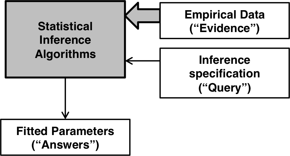
Statistical inference algorithms (e.g. linear models, null-hypothesis tests, etc.) take empirical data (a.k.a. “evidence”) as input, a set of specifications (a.k.a. “query”) and produce fitted parameters (a.k.a. “answers”) as output.

Buried in every statistical inference algorithm are assumptions that can be interpreted as its model of the data generation process. It’s called “inference” because the algorithm finds the model parameters (“answers”) that give the best fit to the empirical data (“evidence”). Examples:

• Linear regression algorithm models data generation as a linear process plus independent Gaussian noise.
• K-means clustering algorithm takes a parameter $K$, and models the data generation process as $K$ centroids spaced reasonably far apart, plus independent Gaussian noise.

What if the evidence doesn’t fit the model of data generation? With statistical inference tools, you need to switch algorithms, or maybe chain them together in some way. Unless you write your own statistical inference algorithms, you can’t programmatically specify the data generation process.

“Math of Thought”: Logic and Programs³

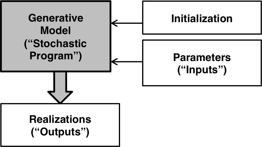
Now we switch our attention from the data to the system that generates the data. Computer programs are the tools we use to simulate the system, taking model parameters and initial conditions as inputs. If there is no randomness in the programs, then the simulations produce the same outputs each run.

Here is an example of two simple programs, one deterministic and one stochastic. Click “run” several times and notice the changes in output.

///fold:
var gauss_legendre_iteration = function(n, a,b,t,p){
var a1 = (a + b) / 2;
if (n > 0) {
gauss_legendre_iteration(
n - 1,
a1,
Math.sqrt(a * b),
t - p * Math.pow(a - a1,2),
2 * p
)
} else {
return Math.pow(a + b,2) / (4 * t)
}
}

var gauss_legendre = function(n){
var a = 1
var b = 1 / Math.sqrt(2);
var t = 1 / 4;
var p = 1;

return gauss_legendre_iteration(n, a,b,t,p);
}
///

var x = uniform(0,1.0);

var pi = gauss_legendre(10); // 10 iterations

print("Deterministic program: Gauss-Legendre algorithm for computing digits of pi\n pi = " + pi + "\n");

print("Stochastic program: A random draw from uniform distribution\n x =" + x);

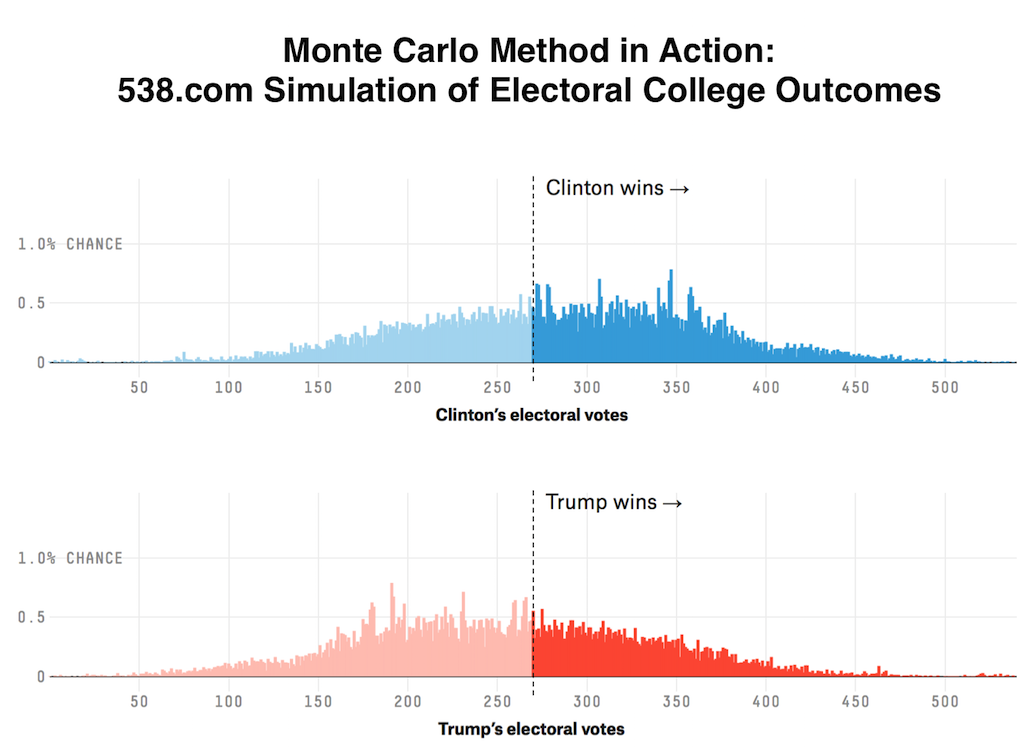
The Monte Carlo method involves running a stochastic program $N$ times and analyzing the distribution of outcomes.

Ordinary programming languages (C, Java, PHP, R, Lisp) are ‘Turing-complete’ because they all the full computational power of a Turing Machine.

---

Endnotes and Credits*

1. ↩ This pithy phrase comes from Joshua Epstein’s presentation: “How to Grow a Mind: Statistics, Structure and Abstraction”

2. ↩ These points are adapted from Avi Pfeffer’s MLconf presentation: “Probabilistic Programming with Figaro”

3. ↩ These diagrams are adapted from cite:pfeffer_practical_2016