Basics of Risk Modeling

This purpose of this chapter is to begin to show how probabilistic programming can be applied in risk analysis and modeling. These models and examples are intentionally basic and toy-like to make them easier to explain and understand. But they should set the stage for the more sophisticated and realistic models in following chapters.

A Simplistic but FAIR Risk Model for Loss Event Risk

The Factor Analysis of Information Risk (FAIR) framework has an ontology as a key element. At the highest level, the ontology looks like this (source: FAIR Institute, developers and promoters of FAIR):

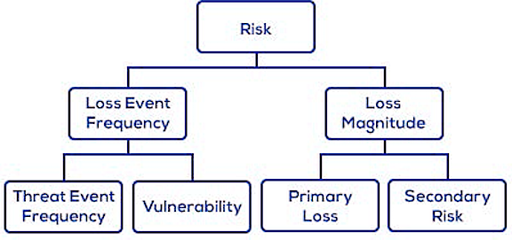
We’ll use this to build a simplistic model of loss event risk.

Note: I call it "simplistic" not as a criticism of FAIR, but for two other reasons. First, we are only looking at this top-level ontology, which abstracts away from all the interesting stuff at ground level. Second, this approach might lead one to develop this model for each and every information asset and each and every threat type. I call this the "Little 'r' approach'" to risk modeling, and I have serious objections to this approach. For a full discussion, see my blog post: "Risk Mangement: Out with the Old! In with the New!".

The simplistic model of risk follows this formula:

$$Risk = Frequency \times Magnitude$$

over some time period, say one year (annualized). If $Frequency$ is 4 times per year and $Magnitude$ is $100, then annualized $Risk$ would be $4 \times \$100 = \$400$. If only risk modeling were so simple! What if $Frequency$ is only “4 times per year” on average, but could be many more or many fewer? What if $Magnitude = \$100$ on average, but could be much higher or a little lower? In otherwords, neither $Frequency$ nor $Magnitude$ are fixed variables, but instead are random variables. This is where we could use some probabilistic modeling to understand the implications.

Let’s assume that the frequency of loss events is governed by a Poisson random process. (The Poisson process is perhaps the simplest model of arrival times and event frequencies.) If the average (mean) number of events per year is 4, then the Poisson distribution looks like this:

var freqModel = Infer({method: "forward", samples: 1000},
    function(){ 
        var f = sample(Poisson({mu : 4}));
        return {"events per year": f};
    });

viz.auto(freqModel);

Both the mode (most frequent) and mean (average) value is 4 per year, but 2 out of 100 years there are zero events, and more rarely there are 10 or more events per year.

Let’s assume that the magnitude of loss is governed by a lognormal distribution.

Lognormal distribution is a good simple assumption. It's always greater than or equal to zero and has a "slightly heavy" "tail. Lognormal distributions are common in nature whenever there are random variables that multiply together to produce some aggregate result. See Life is Lognormal.

Here is a model of lognormal loss magnitude, with $\mu =log(100)$ and and $\sigma = log(3)$.

var magnModel = Infer({method: "forward", samples: 10000},
    function(){ 
        var m = Math.exp(sample(Gaussian({mu : Math.log(100), sigma:Math.log(3)})));
        return {magnitude: m};
    });

print("Magnitude Probability Density Function - Full");
viz.density(magnModel);
print("Magnitude Probability Density Function; range: $0 to $200");
viz.density(magnModel, {bounds: [0,200]});
print("Magnitude Probability Density Function; range: $200 to $4,000");
viz.density(magnModel, {bounds: [200,4000]});

Here we see three visualizations of the magnitude distribution. In the range of $0 to $200, we see that though the mean of this distribution is $100, the mode (most frequent) is a little less than $50. In the range of $200 to $4,000, we see that large losses are not uncommon. Not “Black Swan” territory, but pretty big and a bit surprising if you are only budgeting for $100 per loss event.

Let’s multiply these together to calculate $Risk$, per our simple formula above.

var riskModel = Infer({method: "forward", samples: 10000},
    function(){ 
        var m = Math.exp(sample(Gaussian({mu : Math.log(100), sigma:Math.log(3)})));
        var f = sample(Poisson({mu : 4}));
        var r = f * m;
        return {risk: r};
    });

print("Risk Probability Density Function - Full");
viz.density(riskModel);
print("Risk Probability Density Function; range: $0 to $400");
viz.density(riskModel, {bounds: [0,400]});
print("Risk Probability Density Function; range: $400 to $8,000");
viz.density(riskModel, {bounds: [400,8000]});

The probability density function for $Risk$ is a skew-right with a significant tail (if not actually “heavy”). Looking at the range of $0 to $500, we see the mean at $400, consistent with our previous calculations based on expected (average) values for each. Again, the mode is lower, just below $200. That means you’d see more years with $200 losses than $400, even though $400 is the average over many, many years. The bottom chart show sthe range of $500 to $8,000, and this shows that losses of over $4,000 per year (10X average) are possible, though rare.

So far we have modeled the top three factors in the FAIR ontology, above. Now let’s add the bottom layer of factors.

Threat Event Frequency (TEF) is the frequency (per year) for any event that might trigger the loss, if it succeeds. Vulnerability, in this simplistic model, is the proportion of threat events (a.k.a. attacks) that succeed. Let’s use a Poisson process to model TEF like we did above, with with $mean = 40$ – 10X more frequent than above. For Vulnerability, which must be between 0 and 1.0, let’s use a Beta distribution rather than a point probability (i.e. $v = 0.1$) I chose this one because I’d like to model a vulnerability itself as a random process, which works well most of the time ($v \approx 0$) but occassionally does not ($v >> 0$). Here, the parameters are Beta(1.05,10), which gives $mean \approx 0.1$ and $s.d \approx 0.09$.

var TEFModel = Infer({method: "forward", samples: 1000},
function(){ 
var f = sample(Poisson({mu : 40}));
return {"threat events per year": f};
});

viz.auto(TEFModel);
var vulnModel = Infer({method: "forward", samples: 10000},
    function(){ 
        var v = beta({a : 1.05, b: 10});
        return {vulnerability: v};
    });

print("Vulnerability Probability Density Function");
viz.density(vulnModel);
var samps = repeat(1000,function(){return sample(vulnModel).vulnerability;});
var mean = listMean(samps);
var variance = listVar(samps,mean);
print("Mean = " + mean + "; SD = " + Math.sqrt(variance));

Now we’ll combine these to create a new model for Frequency. But we won’t be multiplying these, as we did in the previous risk model. Why? Because for each threat event (a.k.a. attack), it will either succeed or fail. In this simplistic model, it can’t succeed fractionally. One way to do this: first draw from the TEF distribution to get a value for number of threat events in that simulated year, then we need to flip a biased coin (a.k.a. Bernoulli trial) that many times, with probability of “heads” (success) drawn from the vulnerability distribution. Got it? Maybe or maybe not. Hopefully, the code below will make it more clear.

This way is intuitve, but SLOW (notice only 5 samples):

var freqModel = Infer({method: "forward", samples: 5},
    function(){
        var threatEvents = sample(Poisson({mu : 40})); // this returns an integer
        var vulnerability = beta({a : 1.05, b: 10});   // a real number 0..1, probability of success
        var trials = repeat(threatEvents, function(){
            return flip(vulnerability);
        });
        // this counts the number of successes in the trials
        var successes = reduce(function(x,acc){
                return x == true ? acc + 1 : acc;
            },0,trials);
        return {"loss event frequency" : successes};
});

viz.auto(freqModel);

This may take a long time. Feel free to click cancel.

The following model is much faster, because instead of a nested loop, we sample from Binomial(...), which is the probability of the number of successes in $n$ Bernoulli trials, where probability of trial is $p$. (Notice: 1,000 samples!).

There are three models here for comparison. The first repeats the TEF model. The second uses a point probability: $Vulnerability = 0.1$. The third model uses a Beta(...) distribution for Vulnerability.

var TEFModel = Infer({method: "forward", samples: 1000},
    function(){ 
        var f = sample(Poisson({mu : 40}));
        return {"threat events per year": f};
    });
print("TEF Frequencies")
viz.auto(TEFModel);

var freqModelPoint = Infer({method: "forward", samples: 1000},
    function(){
        // this returns an integer
        var threatEvents = sample(Poisson({mu : 40})); 
        // a real number 0..1, probability of success
        var vulnerability = 0.1;   
        var successes = sample(Binomial({p:vulnerability, n: threatEvents}) );
        return {"loss event frequency" : successes};
});
print("Loss Event Frequencies - Point probability Vulnerability = 0.1")
viz.auto(freqModelPoint);

var freqModel = Infer({method: "forward", samples: 1000},
    function(){
        // this returns an integer
        var threatEvents = sample(Poisson({mu : 40})); 
        // a real number 0..1, probability of success
        var vulnerability = beta({a : 1.05, b: 10});   
        var successes = sample(Binomial({p:vulnerability, n: threatEvents}) );
        return {"loss event frequency" : successes};
});
print("Loss Event Frequencies - Beta Dist. for Vulnerabilities")
viz.auto(freqModel);

Switching to Loss Magnitude, we need to model Primarily Loss and Secondary Risk. We need to decide on the random process for each and then to decide how to combine them. Starting with Primary Loss, let’s assume this is a lognormal distribution, but with a much smaller standard deviation than we modeled above.

var primaryLossModel = Infer({method: "forward", samples: 10000},
    function(){ 
        var m = Math.exp(sample(Gaussian({mu : Math.log(80), sigma:Math.log(1.5)})));
        return {magnitude: m};
});

print("Primary Loss Probability Density Function");
viz.auto(primaryLossModel);

Secondary Risk is a conditional probabilistic loss. In other words, in some loss events, there is no secondary loss, but with some probability there is a secondary loss, which is drawn from a distribution – we’ll assume it is lognormal. Here’s a model:

var secondaryRiskModel = Infer({method: "forward", samples: 10000},
    function(){ 
        var trigger = flip(0.4);
        var loss = trigger 
            ? Math.exp(sample(Gaussian({mu : Math.log(100), sigma:Math.log(3.5)}))) 
            : 0;
    return {magnitude: loss};
}); 

viz.auto(secondaryRiskModel);
viz.density(secondaryRiskModel,{bounds:[0,100]});
viz.density(secondaryRiskModel,{bounds:[100,5000]});

Let’s combine them with addition, and no dependency between them.

var lossMagnitude = Infer({method: "forward", samples: 10000},
    function(){ 
        // primarily loss
        var m = Math.exp(sample(Gaussian({mu : Math.log(80), 
        sigma:Math.log(1.5)})));
        // secondary risk
        var trigger = flip(0.4);
        var s = trigger 
            ? Math.exp(sample(Gaussian({mu : Math.log(100), 
                        sigma:Math.log(3.5)}))) 
            : 0;
        var loss = m + s;
        return {magnitude: loss};
}); 

print("Loss Magnitude Probability Density");
viz.auto(lossMagnitude);
viz.density(lossMagnitude,{bounds:[0,400]});
viz.density(lossMagnitude,{bounds:[400,10000]});

Risk Model V2

Finally, we combine the version 2 model of Loss Event Frequency and Loss Magnitude to get Risk V2.

var lossMagnitude = Infer({method: "forward", samples: 20000},
    function(){ 
        // primarily loss
        var m = Math.exp(sample(Gaussian({mu : Math.log(80), 
        sigma:Math.log(1.5)})));
        // secondary risk
        var trigger = flip(0.4);
        var s = trigger 
                    ? Math.exp(sample(Gaussian({mu : Math.log(100), 
                                        sigma:Math.log(3.5)}))) 
                    : 0;
        var loss = m + s;
        return loss;
}); 

var lossFreq = Infer({method: "forward", samples: 5000},
        function(){
            // this returns an integer
            var threatEvents = sample(Poisson({mu : 40})); 
            // a real number 0..1, probability of success
            var vulnerability = beta({a : 1.05, b: 10});   
            var successes = sample(Binomial({p:vulnerability, n: threatEvents}) );
        return successes;
});


var riskModel = Infer({method: "forward", samples: 50000},
        function(){ 
            // Loss Event Frequency
            var events = sample(lossFreq);

            var risk = sum(
                        repeat(events,function(){return sample(lossMagnitude)})
            );
            return {risk: risk};
}); 

print("Risk Probability Density");
var resultSamples = repeat(5000,
    function () {
        var samp = sample(riskDist);
        return samp.risk;});
var mean = listMean(resultSamples);
var sd = listStdev(resultSamples,mean);
print("Risk Distribution, mean = " + mean + ", std dev = " + sd);

viz.auto(riskDist);
viz.density(riskDist,{bounds:[0,400]});
viz.density(riskDist,{bounds:[400,10000]});
// NOTICE: This takes a lot of execution time because so many samples are
//         are being drawn, in order to get decent estimates in the tail